Cameras lie. Not on purpose. They just see flat surfaces from angles, and angles bend rectangles into trapezoids. For most of what we use cameras for, this doesn't matter. But the moment you want to measure something on that surface (the real distance between two points, the actual size of an object, where on a map a particular pixel falls), the distortion stops being incidental and becomes the whole problem.
This post is about the tool that solves it: homography. We'll cover what it is, the math behind it, how to compute it from a handful of matched points, and offer an interactive demo to play with. Then we'll walk through the project that pulled us into it: estimating the real-world velocity of a moving cart from a single fixed camera.
What is homography?
The word homography comes from Greek: homos (same) and graphein (to write, or draw). Same drawing. And that's a surprisingly accurate name for what it does.
Take a photo of a flat surface straight-on and you see a rectangle. Tilt the camera and you see a trapezoid. The physical object didn't change. The perspective changed. Homography is the mathematical relationship between those two views. It tells you: given a point in one image, where does the same point appear in the other?
What connects the two views is a single 3×3 matrix, usually called H. That's it. Multiply a point by H and you get its corresponding position in the other view.
You might be thinking: "This is just a projective transformation matrix." And yes, that's exactly what it is. For those who haven't thought about transformation matrices in a while, here's how homography fits into the bigger picture.
We have a hierarchy of 2D transformations, where each level adds more flexibility:
Translation moves things around (2 degrees of freedom)
Euclidean/rigid adds rotation (3 DOF)
Similarity adds uniform scaling (4 DOF)
Affine adds shearing and non-uniform scaling (6 DOF)
All of the simpler transformations are special cases of homography. Affine transformations preserve parallel lines. Homography doesn't, which is why parallel lines can appear to converge toward a vanishing point when viewed in perspective. But one property is preserved across all levels: straight lines stay straight. This is what makes homography so useful for working with planar surfaces like floors, walls, documents, and sports fields.
Using homography in practice means computing H. The standard recipe takes a small number of point correspondences — pairs of points where the same physical point shows up in both views, with known coordinates in each — and solves for the matrix that maps one onto the other. H has 9 entries but only 8 of them are independent, and exactly four point correspondences give the information needed to pin those 8 numbers down.
If you want the algebra behind that — why scaling makes one entry redundant, and how four pairs of points give exactly the eight equations needed to solve for H — expand the math section below. Otherwise, skip past it; the rest of the post works on its own.
Computing it in practice
Direct Linear Transform (DLT)
The standard method for computing H is called the Direct Linear Transform. Each point correspondence gives two linear equations in the entries of H, so four correspondences give eight — exactly the right number to solve for the eight independent entries. As long as no three source points are collinear, the system has a unique solution that we can read off directly. At 4 points there's nothing to minimize; the answer is exact.
It gets more interesting when you have more than 4 correspondences (say, hundreds from an automatic feature matcher). The system is overdetermined. With perfect data, the extra equations are redundant: they all agree on the same H. With noisy data (matches off by a few pixels), no single H satisfies all of them exactly. The standard fix is Singular Value Decomposition (SVD), which finds the H that minimizes the total deviation across all the equations in a least-squares sense — falling back to the exact answer when one exists.
RANSAC
DLT works beautifully when your point correspondences are accurate. But what if they're found automatically (say, by a feature matching algorithm) and some of them are wrong?
This is where RANSAC (Random Sample Consensus) comes in. RANSAC doesn't replace DLT; it wraps around it. The algorithm works like this:
Randomly pick 4 point correspondences from your set
Compute H using DLT on just those 4 points
Use that H to transform all other source points and check how close they land to their expected targets
Count how many points agree with this H (the "inliers")
Repeat many times
Keep the H with the most inliers
Recompute H one final time using DLT on all the inliers
The beauty of RANSAC is that even if half your correspondences are wrong, it will eventually stumble upon 4 correct ones, compute a good H, and then identify the rest of the good matches by checking which ones agree. The bad matches get discarded automatically.
In code
And because we live in the age of great open-source libraries, all of this reduces to a few lines of OpenCV:
import cv2
import numpy as np

src_pts = np.array([[x1,y1], [x2,y2], [x3,y3], [x4,y4]], dtype=np.float32)
dst_pts = np.array([[x1_,y1_], [x2_,y2_], [x3_,y3_], [x4_,y4_]], dtype=np.float32)

# Default: least-squares using ALL points (no outlier rejection)
H, status = cv2.findHomography(src_pts, dst_pts)

# With RANSAC for robust estimation (rejects outliers):
H, mask = cv2.findHomography(src_pts, dst_pts, cv2.RANSAC, 5.0)

warped = cv2.warpPerspective(image, H, (width, height))
Decades of geometry research, four lines of code.
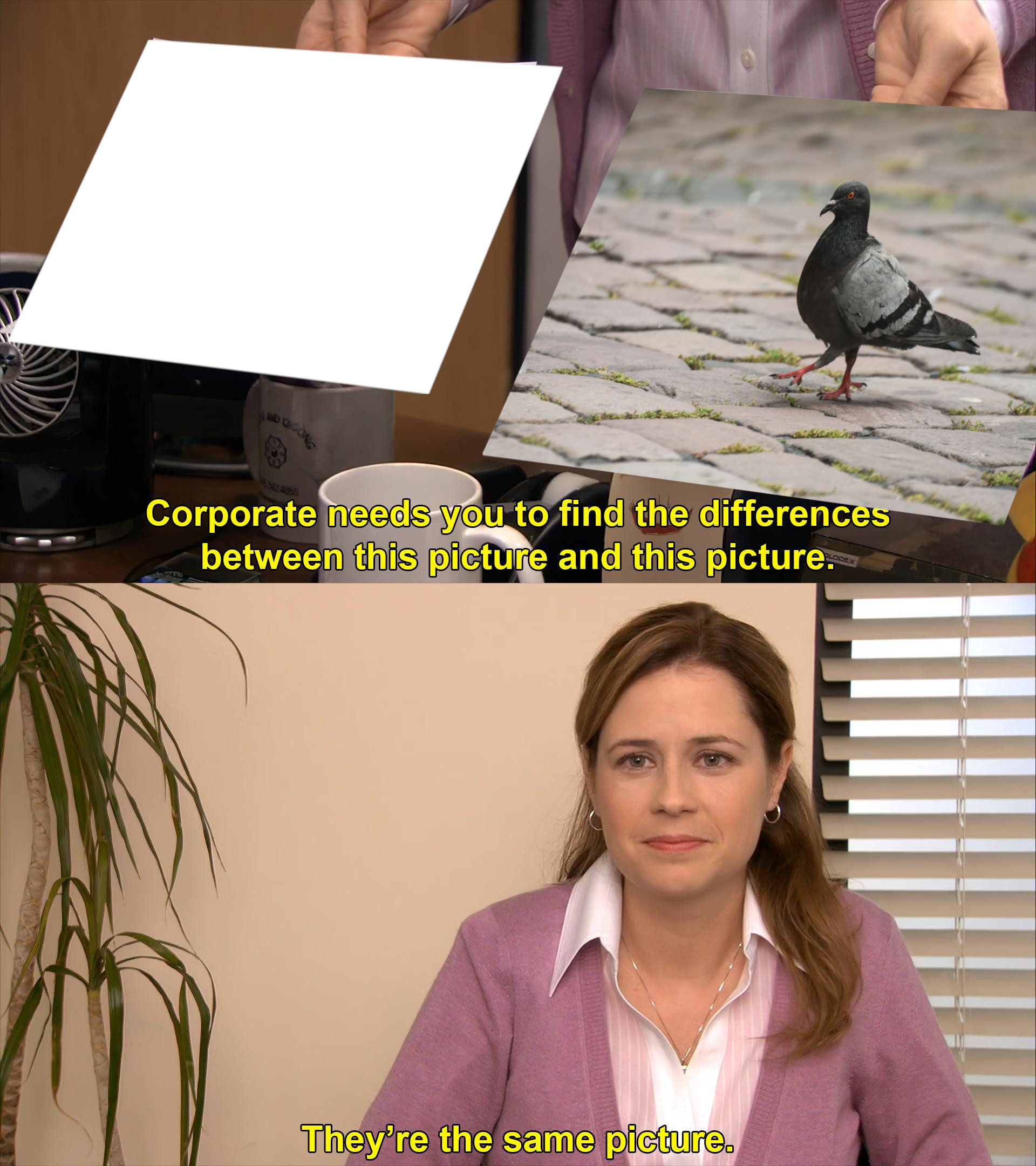
Try it yourself: they're the same picture
DLT is most fun once you can play with it. The demo below is built around the classic they're the same picture meme. On the left is a pigeon. On the right is the meme template, where one frame is already filled with the same pigeon and the other is sitting empty. The job is to pick four corresponding points: corners of the pigeon on the left, corners of the empty frame on the right. DLT solves for the 3×3 matrix that maps point 1 onto point 1, point 2 onto point 2, and so on. Apply it to the pigeon and it snaps into the empty frame. They're the same picture.
A few things worth knowing about what's actually happening under the hood. DLT computes the H that maps your four source points exactly onto your four destination points, but H then warps the entire source plane the same way. If your source points sit on the corners of the pigeon, the warped image fits neatly inside the destination quadrilateral. The 3×3 matrix displayed below the panels is exactly the H that DLT computes, with h33=1 as the normalization, so you can read off all 8 independent parameters of the homography directly.
The Add random warp button gives the pigeon a fresh, gentle perspective distortion. It's the same setup that document scanners and AR apps deal with all the time: a flat thing seen from an awkward angle. Try undoing it: pick the corners of the now-skewed pigeon on the left, the corners of the empty frame on the right, and watch H absorb both the source warp and the destination quadrilateral in a single matrix.
Source — the pigeon
1
2
3
4
Template — the meme
1
2
3
4
Homography matrix H
Click “Compute H & Warp” to see the matrix
How to use
Drag the numbered points on the left to mark four pigeon corners or features.
Drag the matching points on the right onto the empty meme frame.
Click Compute H & Warp to apply the homography.
Add random warp applies a gentle random distortion to the pigeon.
Reset restores the defaults.
Common use cases
What you just did, picking four correspondences and using them to warp an image, is the core building block behind a surprising number of computer vision tools. Image warping is just one example; homography shows up all over the field. Here are a few of the most common applications.
Panorama stitching. Your phone takes overlapping photos, detects common features between them, estimates homographies, and warps everything into a single seamless panorama. This is one of the most classic applications of RANSAC + homography.
Document scanning. Apps like CamScanner and Microsoft Lens detect the four corners of a document, compute H, and warp the image into a clean top-down view. This is DLT in its purest form: four known corners, one transformation, done.
Augmented reality. When you place virtual furniture on your floor using the IKEA app, that object needs to stay anchored to the ground plane as you move the camera. Homography (along with more advanced pose estimation) is what makes that work.
Sports analytics. Broadcast cameras film the pitch at an angle, but analysts want player positions in a top-down tactical view with real-world coordinates. Homography maps from the distorted camera view to the flat field plane.
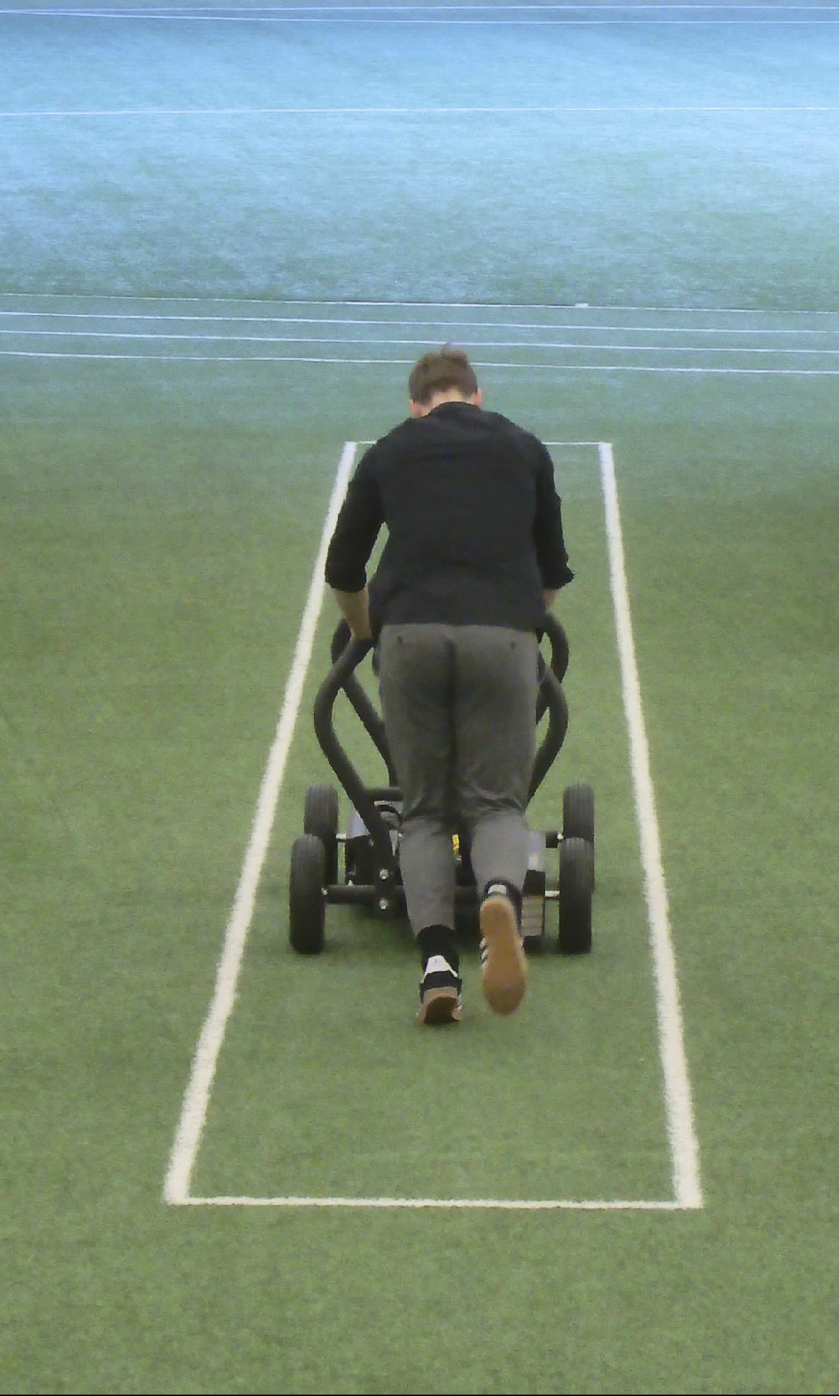
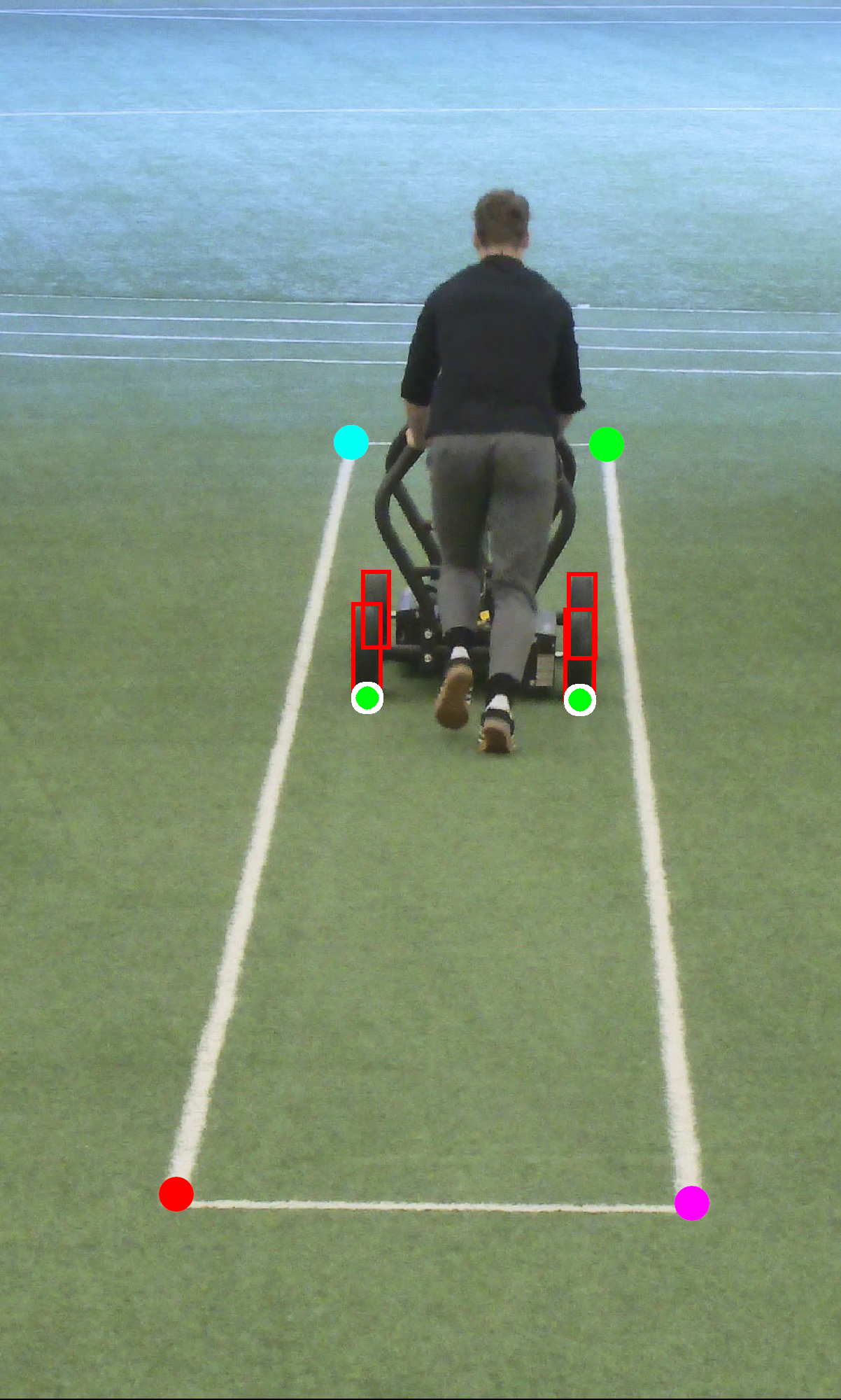
Our use case: computing cart velocity from camera footage
We had a project where we needed to estimate the real-world velocity of a moving cart using a fixed camera. An AI model detected the wheels of the cart in each frame, giving us pixel coordinates. The naive approach would be to track those pixel positions over time and compute velocity from the displacement.
The problem is that pixels are not meters.
The cart was moving away from the camera, deeper into the frame. This is the worst case for naive pixel-based measurement, because perspective compression means that a cart moving 10 pixels far from the camera has covered a much larger physical distance than a cart moving 10 pixels close to the camera. Without correction, the computed velocity would depend on where in the frame the cart happened to be, which is obviously wrong.
The fix was homography. Here's what we did:
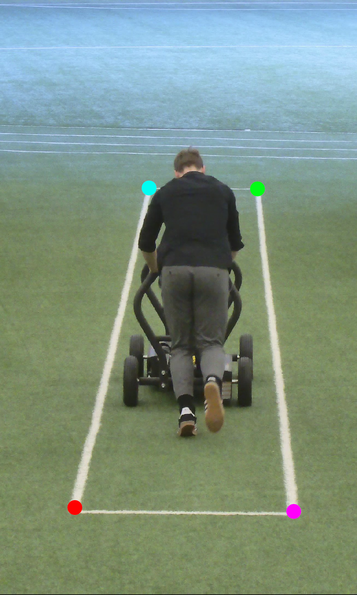
Step 1: Define a reference plane. We identified a rectangle in the scene, a physical structure whose real-world dimensions we knew (we asked the client to measure it). This gave us four correspondences: the pixel coordinates of the rectangle's corners mapped to their known positions in meters.
H=?????????
Step 2: Compute H. With four accurate correspondences, we computed the homography matrix using DLT. Since we had hand-verified annotations of a known physical structure, there was no need for RANSAC. The points were accurate.
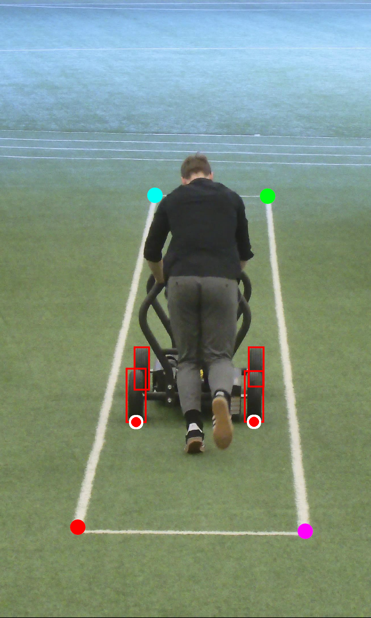
Step 3: Transform wheel positions. For every frame, we took the detected wheel positions in pixel coordinates and multiplied them by H to get their positions in real-world coordinates on the ground plane. This works for any point on the plane, not just within the rectangle, since the homography maps the entire plane.
The key result: after the transformation, measurements came out in real meters everywhere in the image. The pixel-to-meter conversion was correct near the camera and correct far from it. One 3×3 matrix eliminated the perspective distortion problem.
A few caveats
The clean version of homography makes it look like a free lunch. Pick four points, get H, problem solved. In practice there are two failure modes worth knowing about, and they both come from the same fact: a camera doesn't see all of the plane equally well.
Far things are harder to detect. The cart at ten meters covers a small fraction of the pixels it does at three meters. A wheel detector that nails the position up close gets visibly shakier toward the back of the lane, with jumpier bounding boxes and a drifting centroid. Detection noise grows with distance.
Distant pixels cover more ground. This is the part that bites. A one-pixel error near the camera translates to a small physical offset, maybe a centimeter, because the camera resolves the nearby region in fine detail. The same one-pixel error far away can translate to ten or twenty centimeters, because perspective compresses the distant part of the plane onto fewer pixels. Each one of those pixels carries more meters with it.
The two effects line up rather than cancel. Far from the camera you have both a noisier detection and a bigger pixel-to-meter conversion factor, and they multiply, so accuracy degrades fast as the cart moves away. We handled this at setup: the stretch of ground where the velocity actually mattered to us sat close enough to the camera that both detection noise and the pixel-to-meter scaling stayed well within tolerance, so neither effect ended up biting us in practice.
Closing thoughts
What's striking about homography is the leverage. The math has been around for over a century, the algorithm fits in a few lines of code, and OpenCV exposes it as a single function call. In return, you get a bridge between pixel space and the real world for any flat surface: meters from pixels, top-down views from oblique shots, AR objects pinned to the floor, panoramas stitched from your camera roll. A single 3×3 matrix doing the work that would otherwise need extra sensors, careful calibration, or both.
Whenever your data lives on a plane and you need physically meaningful measurements from a camera, the answer is almost always homography. Same drawing, different perspective. Eight numbers do the rest.